The update model

Every algorithm in dynG updates its result with one template: the batch-update framework of thesis Chapter 3 (S M Shovan, Missouri S&T), made concrete by the mechanisms that the six research codes use and the thesis text leaves implicit. This page explains the template, the two families of properties it serves, and how an algorithm maps onto it, with sssp as the worked example. Every algorithm page has a “Template mapping” section in the same shape.

The problem

A graph G_t has a property P_t: shortest-path distances, a cycle histogram, triad counts, labels. A batch Δ of changes arrives (edge insertions and deletions, weight changes; later vertex, hyperedge and incidence changes). The goal is P_{t+1} of G_{t+1} = G_t + Δ, computed from P_t and Δ instead of from scratch.

Given G_t, its property P_t and a batch Δ: Step 1 processes Δ in parallel to find the affected set (the frontier F). Step 2 updates F and produces the next frontier F’ until the frontier is empty. The template is property-agnostic and architecture-agnostic. (thesis Chapter 3)

The template

The thesis states two steps. Reading the six corrected research codes added ten mechanisms (G1-G10) that the two-step description leaves implicit, so the library’s template has more, named steps, always run in this order:

update(problem, graph, batch):
  Step 0   normalize(batch)                  G1  set semantics / net effect / validation
           translate(batch)     [optional]   G7  hypergraph -> line graph, vertex -> edges, ...
           prepare(batch)       [optional]   G1/G2  group by owner, classify improving / invalidating
  Step 1a  before_apply(old view, batch)     G4  reads G_t (e.g. subtract counts that disappear)
  apply    commit                                G_t -> G_{t+1}, exactly once, even for several results
  Step 1b  identify_affected(new view)       G3  roots -> invalidate -> frontier F
           seed(F)              [optional]   G9  initial values for new or invalidated elements
  Step 2   fixed point:     while !is_converged(F): F <- loop(F)          G5, G10
           aggregate delta: delta += count(F, sign = +1, ownership)       G5, G6
  finish   finalize()                        G8  combine, apply deltas, unpack

Written as one line, the template card that heads every algorithm’s page and source:

normalize -> translate -> prepare -> [before_apply -> (AG: count -)] -> commit ->
identify_affected -> seed -> { FP: loop until is_converged | AG: count + } -> finalize

Why each step is separate:

• Step 0 (normalize, translate, prepare) turns the requested operations into the net change under the graph’s batch semantics (upsert or error on an existing edge, what a missing deletion means, self-loops; ADR 0010), and validates ids and weights before anything changes. A batch that fails validation leaves the graph and the result untouched.

• before_apply is the only step that may read the old graph G_t. Aggregate algorithms subtract here the contributions that the batch destroys; they must be counted on G_t, never on G_{t+1} (invariant I1: the library gives the two graph states different view types).

• commit applies the batch once. When several results live on one graph, dyng::update(res, g, batch, r1, r2, ...) runs every result’s Step 0 and before_apply, commits once, then runs every result’s Steps 1 and 2.

• identify_affected and seed build the frontier on G_{t+1}: which elements may have a wrong value now, and what they restart from.

• Step 2 is where the two families differ (below).

• finalize turns the working state into the published result (for sssp: unpack the packed (distance, parent) words) and fills the statistics.

The same names are the profiler stages (<algo>.<hook>, for example sssp.identify_affected), so the time breakdown of every algorithm reads the same way (Profile an update).

Two families of properties

Fixed point (sssp, mosp, hyper_sssp, label_propagation): a value per element. Step 2 iterates: the frontier’s elements update their values, the elements whose values changed propagate to their neighbours, until the frontier is empty (or a tolerance is met, for approximate algorithms). Termination must be guaranteed by construction: a change that can only make values worse (a deleted tree edge) goes through invalidation, never through plain relaxation, which would count to infinity (invariant I3).

Aggregate delta (cycle_count, triad_count): one global number or histogram. P_{t+1} = P_t - (contributions on G_t owned by the deletions) + (contributions on G_{t+1} owned by the insertions). Step 2 is one signed recount around the changed elements, with no iteration. An ownership rule assigns each pattern (a cycle, a triad) to exactly one changed element, so a pattern touched by several changes is counted once (invariant I2).

The four challenges of Chapter 3

Every algorithm page answers the four questions of thesis Chapter 3:

1. Affected-set rule: which elements can change, found from the batch alone?

2. Propagation scope: how far does a change travel, and why does it stop?

3. Correctness under parallelism: how do concurrent updates agree (atomic minima on packed words, owner groups, signed counts) without locks, and with the same result on every backend?

4. Data structure: what container layout makes Steps 1 and 2 cheap?

Worked example: sssp

The update of a shortest-path tree (DynaMOSP’s SOSP update) maps onto the template like this:

Step (profiler stage)	What sssp does
normalize / prepare (sssp.prepare)	validate the batch; find the largest weight; choose the near-far width
commit (sssp.commit)	apply the batch to the graph; classify each change (deletion, weight increase, improvement)
identify_affected (sssp.identify_affected)	roots = heads v of deleted or weight-increased tree edges (u, v); invalidate their subtrees
seed (sssp.seed)	invalidated vertices and insertion heads pull their best (distance, lowest parent id) from their in-neighbours
loop (sssp.loop)	push decreases outward until no distance changes (a near-far worklist on OpenMP)
finalize (sssp.finalize)	unpack distances and parents; count affected

A small case: the graph 0 -> 1 (4), 0 -> 2 (1), 2 -> 1 (2), 1 -> 3 (1), source 0. The tree has dist = (0, 3, 1, 4) with 1 reached through 2. The batch deletes 2 -> 1 and inserts 2 -> 3 (1).

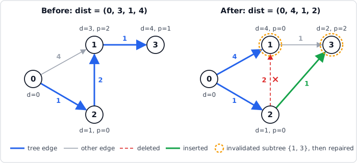
The worked example: the shortest-path tree before the batch (left) and after update() (right). Deleting the tree edge 2 -> 1 invalidates the subtree {1, 3}; seeding repairs vertex 1 through 0 and vertex 3 through the inserted edge 2 -> 3. d is the distance, p the parent. This is the program of A first update in C++ and A first update in Python.

1. Step 0 validates both changes; the commit applies them.

2. identify_affected: the deleted edge 2 -> 1 was a tree edge, so vertex 1 and its subtree {3} are invalidated.

3. seed: vertex 1 pulls its best in-neighbour: 0, at distance 4. Vertex 3 pulls 2 -> 3: distance 2 through vertex 2 (the insertion head is seeded too).

4. loop: no further decrease; the frontier is empty.

5. finalize: dist = (0, 4, 1, 2), parents = (-1, 0, 0, 2), and stats.invalidated == 2.

The profiler shows these steps as stages; in Python:

with dyng.profile(g.resources) as prof:
    st = dyng.sssp.update(g, batch, tree)
print([s.name for s in prof.stages])
# ['sssp.update', 'sssp.prepare', 'sssp.commit', 'graph.apply', 'graph.transpose',
#  'sssp.workspace', 'sssp.identify_affected', 'sssp.seed', 'sssp.loop', 'sssp.finalize']

The answers to the four challenges: (1) subtree invalidation below changed tree edges; (2) only vertices whose distance decreased are expanded, and distances only decrease after the invalidation, so the loop ends; (3) an atomic minimum on a packed (distance, parent) word makes concurrent relaxations agree and gives lowest-id ties on every backend; (4) a CSR with stored in-edges and objective-major weight columns. sssp: dynamic single-source shortest paths has the full mapping.

Engines: framework-composed and fused

The published speeds come from hand-fused GPU kernels (for example MOSP-CUDA’s persistent cooperative kernel). An algorithm may implement Steps 1b-finish as one fused engine for a backend (Tier B); the framework still owns Step 0, the commit, the statistics, the profiler stages and the error checks, so a fused kernel runs inside the same pipeline. The default for new algorithms is Tier A: the steps written with shared operators (advance, filter, invalidate_subtree, group_by_owner, count_delta, …). The option engine (automatic, fused, operators) selects between them where both exist, and a conformance check requires both to give identical results.

The framework itself (problem_base, the enactors, frontiers and operators) is extracted from the first two ported algorithms in milestone M3; it is internal until 0.6.